
Earlier, we studied an application of a first-order differential equation that involved solving for the velocity of an object. In particular, if a ball is thrown upward with an initial velocity of \( v_0\) ft/s, then an initial-value problem that describes the velocity of the ball after \( t\) seconds is given by
This model assumes that the only force acting on the ball is gravity. Now we add to the problem by allowing for the possibility of air resistance acting on the ball.
Air resistance always acts in the direction opposite to motion. Therefore if an object is rising, air resistance acts in a downward direction. If the object is falling, air resistance acts in an upward direction (Figure \( \PageIndex\)). There is no exact relationship between the velocity of an object and the air resistance acting on it. For very small objects, air resistance is proportional to velocity; that is, the force due to air resistance is numerically equal to some constant \( k\) times \( v\). For larger (e.g., baseball-sized) objects, depending on the shape, air resistance can be approximately proportional to the square of the velocity. In fact, air resistance may be proportional to \( v^\), or \( v^\), or some other power of \( v\).

We will work with the linear approximation for air resistance. If we assume \( k>0\), then the expression for the force \( F_A\) due to air resistance is given by \( F_A=−kv\). Therefore the sum of the forces acting on the object is equal to the sum of the gravitational force and the force due to air resistance. This, in turn, is equal to the mass of the object multiplied by its acceleration at time \( t\)(Newton’s second law). This gives us the differential equation
Finally, we impose an initial condition \( v(0)=v_0,\) where \( v_0\) is the initial velocity measured in meters per second. This makes \( g=9.8m/s^2.\) The initial-value problem becomes
The differential equation in this initial-value problem is an example of a first-order linear differential equation. (Recall that a differential equation is first-order if the highest-order derivative that appears in the equation is \( 1\).) In this section, we study first-order linear equations and examine a method for finding a general solution to these types of equations, as well as solving initial-value problems involving them.
A first-order differential equation is linear if it can be written in the form
where \( a(x),b(x),\) and \( c(x)\) are arbitrary functions of \( x\).
Remember that the unknown function \( y\) depends on the variable \( x\); that is, \( x\) is the independent variable and \( y\) is the dependent variable. Some examples of first-order linear differential equations are
\[ \begin (3x^2−4)y'+(x−3)y &=\sin x \\[4pt] (\sin x)y'−(\cos x)y &=\cot x \\[4pt] 4xy'+(3\ln x)y &=x^3−4x. \end\]
Examples of first-order nonlinear differential equations include
These equations are nonlinear because of terms like \( (y′)^4,y^3,\) etc. Due to these terms, it is impossible to put these equations into the same form as Equation \ref.
Consider the differential equation
\[ (3x^2−4)y′+(x−3)y=\sin x. \nonumber \]
Our main goal in this section is to derive a solution method for equations of this form. It is useful to have the coefficient of \( y′\) be equal to \( 1\). To make this happen, we divide both sides by \( 3x^2−4.\)
This is called the standard form of the differential equation. We will use it later when finding the solution to a general first-order linear differential equation. Returning to Equation \ref, we can divide both sides of the equation by \( a(x)\). This leads to the equation
Then Equation \ref becomes
We can write any first-order linear differential equation in this form, and this is referred to as the standard form for a first-order linear differential equation.
Put each of the following first-order linear differential equations into standard form. Identify \( p(x)\) and \( q(x)\) for each equation.
a. Add \( 4y\) to both sides:
In this equation, \( p(x)=4\) and \(q(x)=3x.\)
b. Multiply both sides by \( 4y−3\), then subtract \( 8y\) from each side:
Finally, divide both sides by \( 3x\) to make the coefficient of \( y'\) equal to \( 1\):
This is allowable because in the original statement of this problem we assumed that \( x>0\). (If \( x=0\) then the original equation becomes \( 0=2\), which is clearly a false statement.)
In this equation, \( p(x)=−\dfrac\) and \( q(x)=−\dfrac\).
c. Subtract \( y\) from each side and add \( 4x^2−5\):
Next divide both sides by \( 3\):
In this equation, \( p(x)=−\dfrac\) and \( q(x)=\dfracx^2−\dfrac\).
Put the equation \( \dfrac=5\) into standard form and identify \( p(x)\) and \( q(x)\).
Hint
Multiply both sides by the common denominator, then collect all terms involving \( y\) on one side.
Answer
We now develop a solution technique for any first-order linear differential equation. We start with the standard form of a first-order linear differential equation:
The first term on the left-hand side of Equation \ref is the derivative of the unknown function, and the second term is the product of a known function with the unknown function. This is somewhat reminiscent of the power rule. If we multiply Equation \ref by a yet-to-be-determined function \( μ(x)\), then the equation becomes
The left-hand side Equation \ref can be matched perfectly to the product rule:
Matching term by term gives \( y=f(x),g(x)=μ(x)\), and \( g′(x)=μ(x)p(x)\). Taking the derivative of \( g(x)=μ(x)\) and setting it equal to the right-hand side of \( g′(x)=μ(x)p(x)\) leads to
This is a first-order, separable differential equation for \(μ(x).\) We know \( p(x)\) because it appears in the differential equation we are solving. Separating variables and integrating yields
Here \( C_2\) can be an arbitrary (positive or negative) constant. This leads to a general method for solving a first-order linear differential equation. We first multiply both sides of Equation \ref by this integrating factor by integrating factor \( μ(x).\) This gives
Note that, since the non-zero constant \(C_2\) can be divided out of this equation (as it will appear in every term on both sides), we do not need to use it in this process. That is, we can simply use
The left-hand side of Equation \ref can be rewritten as \( \dfrac(μ(x)y)\).
Next integrate both sides of Equation \ref with respect to \(x\).
\[ \begin \int \dfrac(μ(x)y)dx &=\int μ(x)q(x)dx \\[4pt] μ(x)y &=\int μ(x)q(x)dx \label \end \]
Divide both sides of Equation \ref by \( μ(x)\):
Since \( μ(x)\) was previously calculated, we are now finished. An important note about the integrating constant \( C\): It may seem that we are inconsistent in the usage of the integrating constant. However, the integral involving \( p(x)\) is necessary in order to find an integrating factor for Equation \ref. Only one integrating factor is needed in order to solve the equation; therefore, it is safe to assign a value for \(C\) for this integral. We chose \(C=0\). When calculating the integral inside the brackets in Equation \ref, it is necessary to keep our options open for the value of the integrating constant, because our goal is to find a general family of solutions to Equation \ref. This integrating factor guarantees just that.
Find a general solution for the differential equation \( xy'+3y=4x^2−3x.\) Assume \( x>0.\)
1. To put this differential equation into standard form, divide both sides by \( x\):
Therefore \( p(x)=\dfrac\) and \( q(x)=4x−3.\)
2. The integrating factor is \( μ(x)=e^<\int (3/x)>dx=e^=x^3\).
3. Multiplying both sides of the differential equation by \( μ(x)\) gives us
\[ \begin x^3y′+x^3\left(\dfrac\right)y &=x^3(4x−3) \\[4pt] x^3y′+3x^2y &=4x^4−3x^3 \\[4pt] \dfrac(x^3y) &= 4x^4−3x^3. \end\]
4. Integrate both sides of the equation.
5. There is no initial value, so the problem is complete.
You may have noticed the condition that was imposed on the differential equation; namely, \( x>0\). For any nonzero value of \( C\), the general solution is not defined at \( x=0\). Furthermore, when \( x as \( μ(x)=e^<\int p(x)dx>\). For this \( p(x)\) we get
Find the general solution to the differential equation \( (x−2)y'+y=3x^2+2x.\) Assume \( x>2\).
Hint
Use the method outlined in the problem-solving strategy for first-order linear differential equations.
Answer
Now we use the same strategy to find the solution to an initial-value problem.
Solve the initial-value problem
1. This differential equation is already in standard form with \( p(x)=3\) and \( q(x)=2x−1\).
2. The integrating factor is \( μ(x)=e^<\int 3dx>=e^\).
3. Multiplying both sides of the differential equation by \( μ(x)\) gives
Integrate both sides of the equation:
4. Now substitute \( x=0\) and \( y=3\) into the general solution and solve for \( C\):
Therefore the solution to the initial-value problem is
Solve the initial-value problem \[ y'−2y=4x+3y(0)=−2. \nonumber \]
We look at two different applications of first-order linear differential equations. The first involves air resistance as it relates to objects that are rising or falling; the second involves an electrical circuit. Other applications are numerous, but most are solved in a similar fashion.
We discussed air resistance at the beginning of this section. The next example shows how to apply this concept for a ball in vertical motion. Other factors can affect the force of air resistance, such as the size and shape of the object, but we ignore them here.
A racquetball is hit straight upward with an initial velocity of \( 2~ \text\). The mass of a racquetball is approximately \( 0.0427~ \text\). Air resistance acts on the ball with a force numerically equal to \( 0.5 v\), where \( v\) represents the velocity of the ball at time \( t\).
a. The mass \( m=0.0427~kg,k=0.5,\) and \( g=9.8~m/s^2\). The initial velocity is \( v_0=2 ~m/s\). Therefore the initial-value problem is
Dividing the differential equation by \( 0.0427\) gives
The differential equation is linear. Using the problem-solving strategy for linear differential equations:
Step 1. Rewrite the differential equation as \( \dfrac+11.7096v=−9.8\). This gives \( p(t)=11.7096\) and \( q(t)=−9.8\)
Step 2. The integrating factor is \( μ(t)=e^<\int11.7096dt>=e^.\)
Step 3. Multiply the differential equation by \( μ(t)\):
Step 4. Integrate both sides:
Step 5. Solve for \( C\) using the initial condition \( v_0=v(0)=2\):
Therefore the solution to the initial-value problem is
b. The ball reaches its maximum height when the velocity is equal to zero. The reason is that when the velocity is positive, it is rising, and when it is negative, it is falling. Therefore when it is zero, it is neither rising nor falling, and is at its maximum height:
Therefore it takes approximately \( 0.104\) second to reach maximum height.
c. To find the height of the ball as a function of time, use the fact that the derivative of position is velocity, i.e., if \( h(t)\) represents the height at time \( t\), then \( h′(t)=v(t)\). Because we know \( v(t)\) and the initial height, we can form an initial-value problem:
Integrating both sides of the differential equation with respect to \( t\) gives
Solve for \( C\) by using the initial condition:
After \( 0.104\) second, the height is given by
The weight of a penny is \(2.5\) grams (United States Mint, “Coin Specifications,” accessed April 9, 2015, www.usmint.gov/about_the_mint. specifications), and the upper observation deck of the Empire State Building is \( 369\) meters above the street. Since the penny is a small and relatively smooth object, air resistance acting on the penny is actually quite small. We assume the air resistance is numerically equal to \( 0.0025v\). Furthermore, the penny is dropped with no initial velocity imparted to it.
Set up the differential equation the same way as Example \(\PageIndex\) . Remember to convert from grams to kilograms.
Answer
c. \(\displaystyle \lim_v(t)=\lim_(9.8(e^−1))=−9.8 \text < m/s>≈−21.922\) mph
A source of electromotive force (e.g., a battery or generator) produces a flow of current in a closed circuit, and this current produces a voltage drop across each resistor, inductor, and capacitor in the circuit. Kirchhoff’s Loop Rule states that the sum of the voltage drops across resistors, inductors, and capacitors is equal to the total electromotive force in a closed circuit. We have the following three results:
1. The voltage drop across a resistor is given by
where \( R\) is a constant of proportionality called the resistance, and \( i\) is the current.
2. The voltage drop across an inductor is given by
where \( L\) is a constant of proportionality called the inductance, and \( i\) again denotes the current.
3. The voltage drop across a capacitor is given by
where \( C\) is a constant of proportionality called the capacitance, and \( q\) is the instantaneous charge on the capacitor. The relationship between \( i\) and \( q\) is \( i=q′\).
We use units of volts \( (V)\) to measure voltage \( E\), amperes \( (A)\) to measure current \( i\), coulombs \( (C)\) to measure charge \( q\), ohms \( (Ω)\) to measure resistance \( R\), henrys \( (H)\) to measure inductance \( L\), and farads \( (F)\) to measure capacitance \( C\). Consider the circuit in Figure \( \PageIndex\).
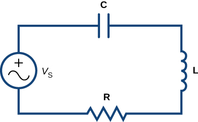
Applying Kirchhoff’s Loop Rule to this circuit, we let \( E\) denote the electromotive force supplied by the voltage generator. Then
Substituting the expressions for \( E_L,E_R,\) and \( E_C\) into this equation, we obtain
If there is no capacitor in the circuit, then the equation becomes
This is a first-order differential equation in \( i\). The circuit is referred to as an LR circuit.
Next, suppose there is no inductor in the circuit, but there is a capacitor and a resistor, so \( L=0, \, R≠0,\) and \( C≠0.\) Then, since \(q′ = i\), Equation \ref can be rewritten as
which is a first-order linear differential equation in \(q\). This is referred to as an RC circuit. In either case, we can set up and solve an initial-value problem.
A circuit has in series an electromotive force given by \( E=50\sin 20tV,\) a resistor of \( 5Ω\), and an inductor of \( 0.4H\). If the initial current is \( 0\), find the current at time \( t>0\).
We have a resistor and an inductor in the circuit, so we have an LR circuit and can use Equation \ref. The voltage drop across the resistor is given by \( E_R=Ri=5i\). The voltage drop across the inductor is given by \( E_L=Li′=0.4i′\). The electromotive force becomes the right-hand side of Equation \ref. Therefore Equation \ref becomes
\[ 0.4i′+5i=50\sin 20t. \nonumber \]
Dividing both sides by \( 0.4\) gives the equation
\[ i′+12.5i=125\sin 20t. \nonumber \]
Since the initial current is 0, this result gives an initial condition of \( i(0)=0.\) We can solve this initial-value problem using the five-step strategy for solving first-order differential equations.
Step 1. Rewrite the differential equation as \( i′+12.5i=125\sin 20t\). This gives \( p(t)=12.5\) and \( q(t)=125\sin 20t\).
Step 2. The integrating factor is \( μ(t)=e^<\int 12.5dt>=e^\).
Step 3. Multiply the differential equation by \( μ(t)\):
Step 4. Integrate both sides:
Step 5. Solve for \( C\) using the initial condition \( i(0)=0\):
Therefore the solution to the initial-value problem is
The first term can be rewritten as a single cosine function. First, multiply and divide by \( \sqrt=50\sqrt\):
Next, define \( φ\) to be an acute angle such that \( \cos φ=\dfrac>\). Then \( \sin φ=\dfrac>\) and
Therefore the solution can be written as
The second term is called the attenuation term, because it disappears rapidly as \( t\) grows larger. The phase shift is given by \( φ\), and the amplitude of the steady-state current is given by \( \dfrac>\). The graph of this solution appears in Figure \( \PageIndex\):
![A graph of the given solution over [0, 6] on the x axis. It is an oscillating function, rapidly going from just below -5 to just above 5.](https://math.libretexts.org/@api/deki/files/12453/8.5.1.png?revision=1)
A circuit has in series an electromotive force given by \( E=20\sin 5t\) V, a capacitor with capacitance \( 0.02F\), and a resistor of \( 8Ω\). If the initial charge is \( 4C\), find the charge at time \( t>0\).
Hint
Use Equation \ref for an RC circuit to set up an initial-value problem.
Answer
integrating factor any function \(f(x)\) that is multiplied on both sides of a differential equation to make the side involving the unknown function equal to the derivative of a product of two functions linear description of a first-order differential equation that can be written in the form \( a(x)y′+b(x)y=c(x)\) standard form the form of a first-order linear differential equation obtained by writing the differential equation in the form \( y'+p(x)y=q(x)\)
This page titled 8.5: First-order Linear Equations is shared under a CC BY-NC-SA 4.0 license and was authored, remixed, and/or curated by Gilbert Strang & Edwin “Jed” Herman (OpenStax) via source content that was edited to the style and standards of the LibreTexts platform.